Condition tables are a data-oriented approach to Decision tables. Decision
tables are a method by which you can generate flow control with a table,
mapping a vector of predicates to a set of outcomes or destinations. In
decision tables, each row has a predicate - a logical statement, such as
isTrue, isFalse, null, or some boolean returning function on the data present
in the column, such as ![]() for numbers, or contains( "win" ) for strings.
Decision tables aren't entirely like standard flow control statements, as they
can lead to multiple outcomes. We will see that a condition table query can
also end up being true for multiple outcomes, or even have no matching rows.
for numbers, or contains( "win" ) for strings.
Decision tables aren't entirely like standard flow control statements, as they
can lead to multiple outcomes. We will see that a condition table query can
also end up being true for multiple outcomes, or even have no matching rows.
Condition tables are similar to Decision tables, except they have some
restrictions that allow for easier optimisation. All the input columns in a
condition table query are boolean. If you are familiar with decision tables,
this might seem like a limiting constraint, however if you need to check that ![]() , then you can do that before it enters the query. Also, unlike decision
tables, each row in a condition table doesn't have a function to call, but
instead a table reference to output to if there is a match on the conditions.
These simple constraints allow for existence-based-processing of the result
tables, thus reducing the instruction cache misses of the more traditional
database oriented decision table approach, and also allows the driving of event
tables so that conditions can trigger events on subscribed entities.
, then you can do that before it enters the query. Also, unlike decision
tables, each row in a condition table doesn't have a function to call, but
instead a table reference to output to if there is a match on the conditions.
These simple constraints allow for existence-based-processing of the result
tables, thus reducing the instruction cache misses of the more traditional
database oriented decision table approach, and also allows the driving of event
tables so that conditions can trigger events on subscribed entities.
For each component involved in the condition table operation, you generate the boolean values into the condition table input. Generating each boolean value from the data in this fashion can utilise the struct-of-arrays format much better, as the predicate can run as a tiny kernel over the streaming data. In a traditional array-of-structs format, this technique wouldn't improve performance or increase cache-line utilisation, so unless you're testing your code on well oriented data, this whole preprocessing step might be worse than pointless. If your data is organised by concept, such as in an object oriented class, then you might end up loading in the same data multiple times to prepare the input table. As each kernel may be accessing only a few bytes of a structure at a time, this will waste memory bandwidth.
Once the condition input is prepared, we then prepare the transform. The transform consists of a set of query arrays and an output. The output will be multiple tables, each query array can point to any of the output tables, which means that an entry can end up in more than one table, and can be put into a table more than one time based on how the output table is organised. Sometimes, an entity will want to only act on the first matching decision point (this would be a way to implement behaviour trees), sometimes a component will want to include multiple matches (this would be a way to implement scoring points).
The condition table is made up of rows, each row has a query array that consists of one or more tri-state columns with possible values of { isTrue, isFalse, null }. To match with an input, all query array columns must match. In effect, an and over all the element queries. The null entry will always return true. With this, it is possible to build up any query you would normally do on your data.
The decision table approach is another form of taking what is normally a singular entity approach and flipping it on its head. Now we are aware of the idea of a structure of arrays, we can start to see other areas of code that previously were being driven by a multiple individual entities entering into update functions and calling things based on their own data, and causing the processor to change direction and try to keep up with the winding trail set by all the selfish entities. If every entity needs to do an update, then effectively no individual entity needs to do an update. Components need to update, and if instead of running an update over each and every entity in your application, you run a component update over every component manager, then you're moving from a data driven mess to a stream processing or flow based programming paradigm. Each of these approaches has benefits, but the difficulty in using them in the past has been how to begin to do it when starting with an object oriented data layout. If your data is already organised as structures of arrays (or indeed component managers of arrays of transform related data), then the flow based techniques for transforming data don't need to be shoe-horned in.
Because we have moved the decisions out of the instances, we are in a position to do more at the same time. A wary object-oriented programmer might assume that each decision table applies to only one set of entities, or one set of queries, but the truth is far more parallel. Once you have moved away from entities being a type, and instead let them be implicit on their components, you find that you can process a very large number of apparently disparate entities at the same time. As you build your application's update function, you find that you need to make decisions for components, update components based on those decisions, and sometimes iterate over that sequence a few times. At no point are you limited to one entity at a time, or even one component at a time unless you build in dependencies into your transform chain.
Moving away from single entity processing is also good if you want to offload your core application code onto a compute shader. As long as you maintain your data in simple arrays inside the components, then there will likely be very little currying of data into a shader ready format. If you make sure your processing is stateless, as in it does not accumulate or modify global state, or reference other elements in the stream in a random access fashion, then it's very likely you will be able to convert your code to a compute kernel. At this point, you will have left the general purpose CPU to scheduling the operations, and joining tables. These are the only jobs still not easily handled by a stateless streaming approach.
With all this raw data moving around, some may think that it would be harder to debug than a human friendly object-oriented code layout. Indeed, some developers think that you need to understand the data in a problem centric way in order to figure out what is causing a bug, however, normally a bug is where the implementation did what was written, not what was meant, and that can usually be found through understanding what is going on inside the software, and not the problem that was being solved by it. Most bug slaying involves understanding what the computer was doing before it did the unexpected. It is hardly ever about understanding the design, or the concepts represented by the classes. It is very unlikely that your bug exists in something as high level as the fact that a house is not a car.
For example, if you have a bug where a specific mesh is being culled, you might think that you need to see the data about the entity that renders that mesh all in one place. You may think that otherwise you could spend a lot of time traversing data structures in a watch window just to find out in what state an object was, that caused it to flip its visible bit to false. This human view of the data may seem important to many seasoned developers, but it's false reasoning based on how difficult it is to debug and reason about data structures inside an object-oriented program. We're used to thinking about our data as objects, but our data is not objects, it's data.
If your code is data-oriented, with checkpoints between each transform, it becomes very easy to log any changes and their reason why. It even becomes simpler to rerun transforms in order to find out what conditions caused them to change. If you are using condition tables, you can run the condition check multiple times to figure out what caused them to emit or not emit output rows. If you keep the development stream-oriented, that is, no mutable state or in-place modification, then you can even allow for rolling back a lot of your program in order to find the original cause of any bad state. We can roll back when we don't have global state mutation because any previous data implies a state. As long as you don't modify the stream, but instead generate a new one as you make your way through your updates, you can always look back and see what caused the change, or at least see where the data didn't match expectation.
If you think about things like meshes as being objects that have state, then you are going to worry about how data got into a particular state. Most object oriented developers fear that without the problem domain borders, then states may get lost in one of the myriad anonymous transforms that affect the data streaming through the system, however, this is only because Object-oriented design allows or even enforces the dangerous practice of hidden data and mutable state. As it is relatively easy to hook an event handler to any table insert, adding logging for bad state changes is very easy, and if you keep your transforms deterministic, it becomes highly repeatable. In some languages there are virtual machines that allow for complete rollback of the program. There is a JVM that maintains historic state, and Microsoft's CLR provides the ability to go back in time for some of its languages. If you program your game with condition tables, thorough logging, and a deterministic set of transforms, you can have game state rollback in a high performance language such as C++.
With this information at hand, it can be safe to assume that for the normal practice of debugging, which is figuring out how an object got into a particularly bad state, working within a well formed data oriented code base would make debugging easier, not harder.
Due to the restrictions imposed on their use, condition tables have the opportunity to be realised in branch free or heavily optimised code. Depending on the number of rows in the decision table, it might be possible to optimise the query by output, but normally the query can be optimised by input. We will see more of this choice of rows vs columns in chapter ref:example.
The first thing we do is generate a truth value from the conditions and the query array. Remember the query array is made up of isTrue, isFalse, and null values. We need to generate, from an array of booleans, a single boolean result. Logically, we can produce this by xoring the inputs with the isFalse elements, and then oring in the null entries. Once we have this final array, we only need to check that all elements are true to find the entire query to be true.
If we allow for our pre-processor to produce bitmasks of input values, then we can produce a pair of bit masks that generate the kind of result we need. First, we prepare the ignore mask, this mask contains a high bit wherever we don't care about the input value. Naturally, all null fields can be converted to 1s, and so can any bits higher than the maximum query entry. The second mask is the falsity masks, and is true if the query array tri-state is isFalse. These masks are now the xor and ignore masks.
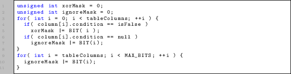
Next, prepare the input as a list of boolean values. If we have well formed data, we can assume that we have already built our inputs as bit fields, but if our data is still object oriented, or at least still arrays of structures, then we will probably do this step inline with reading each structure from the array of structures.
![\begin{lstlisting}
foreach( row in table ) {
unsigned int values = 0;
for( int...
...bleColumns; ++i ) {
if( row[i] )
values \vert= BIT( i );
}
}
\end{lstlisting}](img17.png)
Once you have your inputs transformed into the array of bit fields, you can run them through the condition table. If they are an array of structures, then it's likely that caching the inputs into a separate table isn't going to make things faster, so this decision pass can be run on the bit field directly. In this snippet we run one bit field through one set of condition masks.
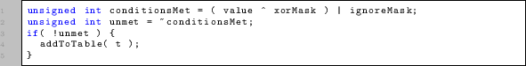
The code first XORs the values so the false values become true for all the cases where we want the value to be false. Then we OR with the ignore so that any entries we don't care about become true and don't falsely break the condition. Once we have this final value, we can be certain that it will be all ones in case of a match, and will have some zeros if it is a miss. An if using the binary-not of the final value will suffice to prove the system works, but we can do better.
Using the conditionsMet value, we can generate a final mask onto an arbitrary value.
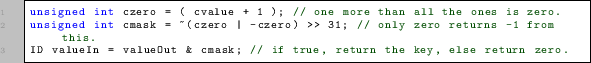
Now, we can use this value in many ways. We can use it on the primary key, and add this key to the output table, and providing a list table that can be reduced by ignoring nulls, we have, in effect, a dead bucket. If we use it on the increment counter, then we can just add an entry to the end of the output table, but not increase the size of the output table. Either way, we can assume this is a branchless implementation of an entry being added to a table. If this was an event, then a multi-variable condition check is now branchlessly putting out an event. If you let these loops unroll, then depending on your platform, you are going to process a lot more data than a branching model will.